
For a simple exercise to understnad one-way ANOVA, I will use the data set red.cell.folate from the package ISwR (see the book “Introductory Statistics with R” by Peter Dalgaard) but will also generate our own data.
kbtools::libmgr("l", c("kbtools", "ISwR", "ggplot2", "reshape2"))
set.seed <- 117
head(red.cell.folate)
## folate ventilation
## 1 243 N2O+O2,24h
## 2 251 N2O+O2,24h
## 3 275 N2O+O2,24h
## 4 291 N2O+O2,24h
## 5 347 N2O+O2,24h
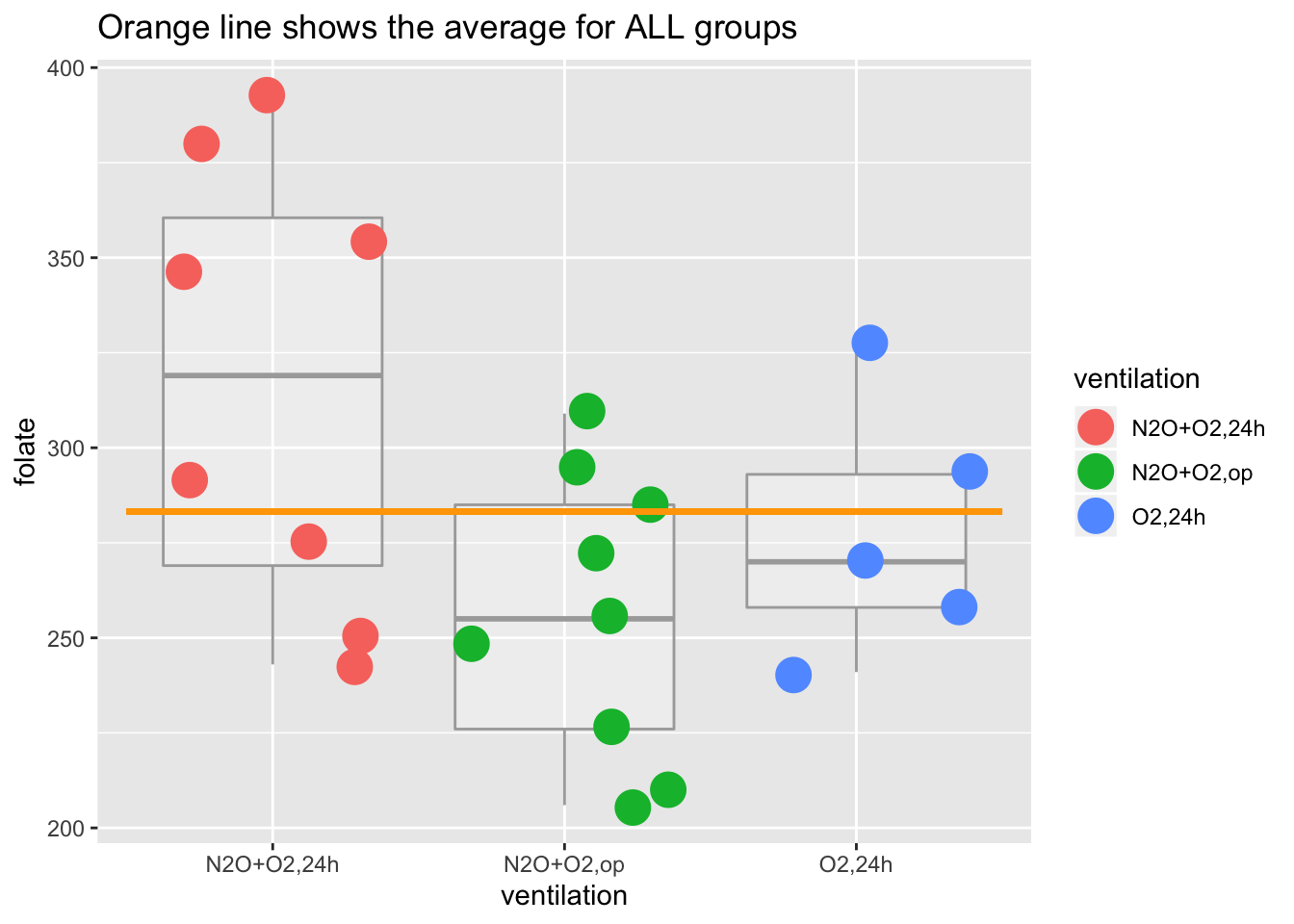
## 6 354 N2O+O2,24hmean(red.cell.folate$folate)## [1] 283.2273ggplot(red.cell.folate) +
geom_boxplot(aes(ventilation, folate), alpha=I(1/4), color="darkgray") +
geom_jitter(aes(ventilation, folate, color=ventilation), size=6) +
geom_segment(aes(x=0.5, xend=3.5, y=mean(folate), yend=mean(folate)), color="orange", size=1) +
labs(title="Orange line shows the average for ALL groups")
And now (drum roll) … it’s time to run the ANOVA
with(red.cell.folate, anova(lm(folate ~ ventilation)))## Analysis of Variance Table
##
## Response: folate
## Df Sum Sq Mean Sq F value Pr(>F)
## ventilation 2 15516 7757.9 3.7113 0.04359 *
## Residuals 19 39716 2090.3
## ---
## Signif. codes: 0 '***' 0.001 '**' 0.01 '*' 0.05 '.' 0.1 ' ' 1Let’s look at what this ANOVA table means.
A bit of background first. In a set of multiple groups, each observation can be linked to the mean of its own group and that group mean can be linked to the mean of all observations (a.k.a. “the grand mean”) so that \[x_{ij}=(x_{ij}-\bar{x}_{i})+(\bar{x}_i-\bar{x})+\bar{x}\] which corresponds to \[x_{ij}=\mu + \alpha_i + \epsilon_{ij}\] where the error terms \(\epsilon_{ij}\) are independent and have the same distribution \[\epsilon_{ij}\sim N(0,\sigma^2)\]
The null hypothesis that all groups are the same implies that all \(\alpha_{i}\) are zero.
The total sum of squares (a.k.a. variation or SSD) equals the SSD “between” groups plus “within” groups \[SSD_{total}=SSD_{B}+SSD_{W}\] The first row in the ANOVA table above is the SSD “between” groups, labeled by the “treatment” or “grouping” factor. The last row is the “within” groups SSD is also known as “residuals” or “errors.”
| SSD component | name | rows | a.k.a. |
|---|---|---|---|
| \(SSD_{B}\) | “between groups” | first (k-1) | treatment, grouping |
| \(SSD_{W}\) | “within groups” | last | residuals, error |
The sums (SSDs) can and should be normalized by their respective degrees of freedom (df) to calculate mean squares. If N is the total number of observations and k is the number of groups, the df for \(SSD_{B}\) is k-1 and for \(SSD_{W}\) is N-k. Therefore
\[ \begin{aligned} \ MS_{B} = \frac{SSD_{B}}{k-1} \\ \ MS_{W} = \frac{SSD_{W}}{N-k} \\ \end{aligned} \]
The \(MS_{W}\) is the pooled variance from combining the individual group variances and is thus an estimate of \(\sigma^2\). If there is no group effect, \(MS_{B}\) will be approximately equal to \(MS_{W}\) (and thus also provide an estimate of \(\sigma^2\)), but if there is a group effect, \(MS_{B}\) will tend to be larger.
The F statistic is \(\frac{MS_{B}}{MS_{W}}\). Under the null hypothesis, F is 1, or a little greater, due to random effects (by the way, this test is one-sided). In the case above \(F=\frac{7758}{2090} = 3.71\).
You reject the null if F is larger than the 95% quantile of an F distribution with k-1 and N-k degrees of freedom, referred to as \(F_{k-1,N-k}\) (in this case, k=3 and N=22).
Just because we can, let’s see what such an F distribution looks like
fdist <- data.frame(F = rf(1000, 2, 19))
ggplot(fdist) + geom_histogram(aes(F), binwidth=prettyb(fdist$F), fill = "steelblue") +
geom_segment(x = qf(.95,2,19), xend = qf(.95,2,19), y=0, yend=50, color="red", size=1) +
annotate("text", x=3.5, y=55, label="95th percentile", size=5, color="red") +
scale_x_continuous(limits = c(0, 8), breaks = seq(0, 8, 1))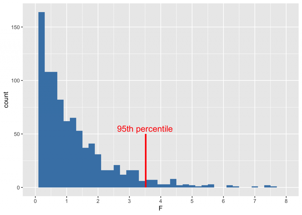
Because \(F=3.71\) is larger than \(qf(.95, 2, 19) = 3.5218933\), we reject the null hypothesis, and conclude that the population means are likely different. Another way of putting this is that \(p = 1-pf(3.71, 2, 19) = 0.0435697\).
Let’s look now at an artificial data set
I love generating datasets that are vaguely medicine-related. Here is one:
n <- 10
age <- rnorm (n, 50, 10)
df <- data.frame(age= age,
                 a= (2 * age + rnorm(n, 0, 40)),
                 b= rnorm(n, 100, 20),
                 c= age * rbeta(n, 1, 5),
                 d=(age/8)^2)#; head(df)
ggplot(df) +
  geom_point(aes(age,a), color="red", size=6, alpha=I(1/1)) +
  geom_point(aes(age,b), color="green", size=6, alpha=I(1/1)) +
  geom_point(aes(age,c), color="blue", size=6, alpha=I(1/1)) +
geom_point(aes(age,d), color="yellow", size=6, alpha=I(1/1)) 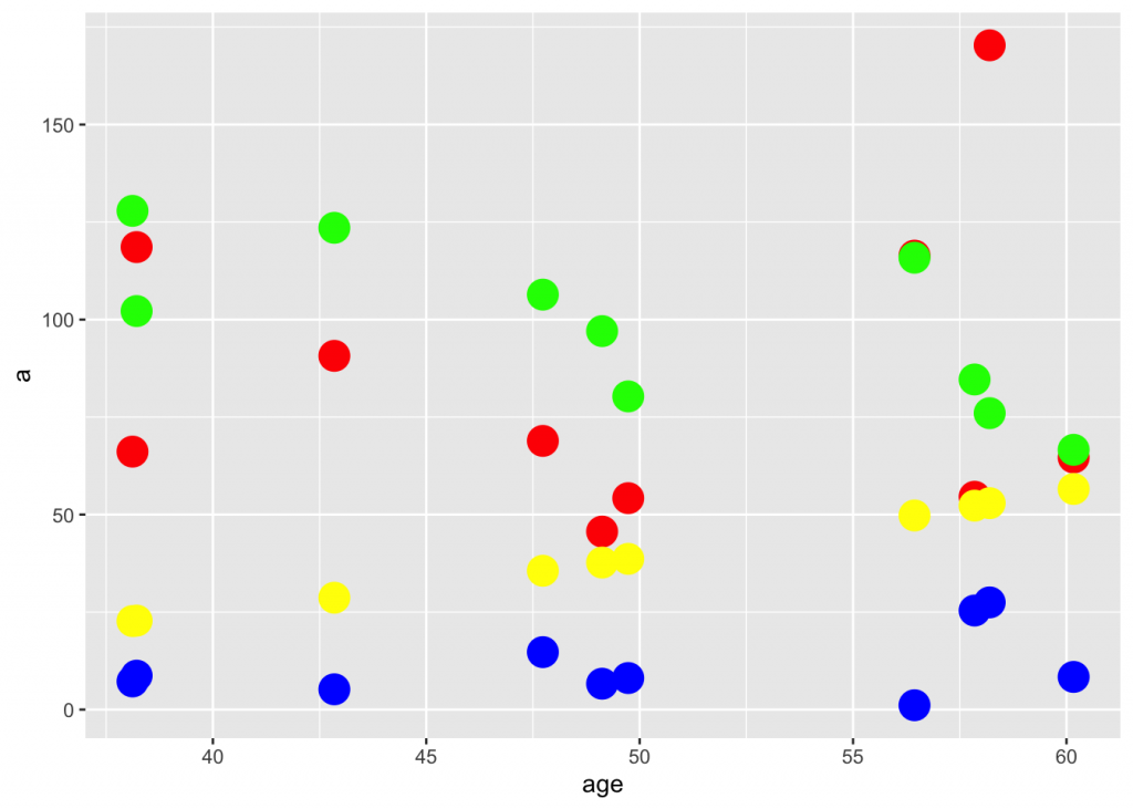
attach(df)The data frame presented this way is not suitable for an ANOVA, because the data has to be molten (a tidyverse concept). A beginner temptation is to run
anova(lm(a~age))## Analysis of Variance Table
##
## Response: a
## Df Sum Sq Mean Sq F value Pr(>F)
## age 1 170.7 170.71 0.0996 0.7603
## Residuals 8 13707.5 1713.44anova(lm(b~age))## Analysis of Variance Table
##
## Response: b
## Df Sum Sq Mean Sq F value Pr(>F)
## age 1 1944.7 1944.7 7.9021 0.02281 *
## Residuals 8 1968.8 246.1
## ---
## Signif. codes: 0 '***' 0.001 '**' 0.01 '*' 0.05 '.' 0.1 ' ' 1The above two analyses do NOT describe a grouping of data, but a linear regression of the effect (a or b) on the predictor variable (age). The df=1 for the effect is a telltale sign! (Dalgaard, p. 130)
You need to melt the data frame
df2 <- melt(df, id="age"); colnames(df2)[2] <-"subgroup"#;head(df2); tail(df2)
ggplot(df2) +
  geom_boxplot(aes(subgroup, value, color=subgroup),  size=1, alpha=I(1/2), color="darkgray", fill="lightgray") +
  geom_jitter(aes(subgroup, value, color=subgroup), size=8, alpha=I(3/4)) +
  geom_segment(aes(x=0.5, xend=4.5, y=mean(value), yend=mean(value)), color="orange", size=2)+
  labs(title="Orange line shows the average for all groups")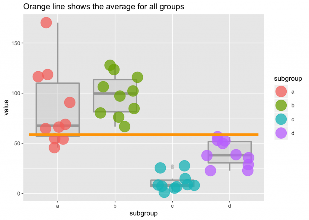
attach(df2)anova(lm(value ~ subgroup)) # NOT age ~ subgroup## Analysis of Variance Table
##
## Response: value
## Df Sum Sq Mean Sq F value Pr(>F)
## subgroup 3 48456 16151.9 29.211 9.416e-10 ***
## Residuals 36 19906 552.9
## ---
## Signif. codes: 0 '***' 0.001 '**' 0.01 '*' 0.05 '.' 0.1 ' ' 1Which is quite obviously significant, but if you are anal and want to run the numbers, \(p = 1-pf(\frac{MS_{B}}{MS_{W}}, k-1, N-k)\).
Pairwise comparisons and multiple comparisons
The F test suggests that the groups are not the same, but will not tell where the difference lies. For that one needs to do pairwise or multiple comparisons.
summary (lm(value ~ subgroup))##
## Call:
## lm(formula = value ~ subgroup)
##
## Residuals:
## Min 1Q Median 3Q Max
## -39.363 -16.329 -2.756 12.677 85.312
##
## Coefficients:
## Estimate Std. Error t value Pr(>|t|)
## (Intercept) 85.010 7.436 11.432 1.55e-13 ***
## subgroupb 13.034 10.516 1.239 0.223215
## subgroupc -73.714 10.516 -7.010 3.19e-08 ***
## subgroupd -45.241 10.516 -4.302 0.000124 ***
## ---
## Signif. codes: 0 '***' 0.001 '**' 0.01 '*' 0.05 '.' 0.1 ' ' 1
##
## Residual standard error: 23.51 on 36 degrees of freedom
## Multiple R-squared: 0.7088, Adjusted R-squared: 0.6846
## F-statistic: 29.21 on 3 and 36 DF, p-value: 9.416e-10The intercept is the mean of the first group, whereas the other two coefficients describe the difference between the given group and the first one.
The p values compare the groups to the first group, but groups 2…k are not compared between themselves. To compare all groups, one needs to adjust for p value inflation, using the Bonferroni correction.
pairwise.t.test(value, subgroup, p.adj="bonferroni")##
## Pairwise comparisons using t tests with pooled SD
##
## data: value and subgroup
##
## a b c
## b 1.00000 - -
## c 1.9e-07 4.9e-09 -
## d 0.00074 1.7e-05 0.06180
##
## P value adjustment method: bonferroniUnequal variance
The typical one-way ANOVA relies on an assumption of equal variance for all groups. In the common scenario when that is not likely to be correct, do not use the pooled standard deviation:
pairwise.t.test(value, subgroup, p.adj="bonferroni", pool.sd=F)##
## Pairwise comparisons using t tests with non-pooled SD
##
## data: value and subgroup
##
## a b c
## b 1.00000 - -
## c 0.00109 2.5e-07 -
## d 0.03220 1.1e-05 0.00014
##
## P value adjustment method: bonferroniWhat if you are unsure about the variances in your groups?
Run the Bartlett test, which evaluates for homogeneity of variance (i.e. the homoscedasticity) of the samples.
bartlett.test(value~subgroup)##
## Bartlett test of homogeneity of variances
##
## data: value by subgroup
## Bartlett's K-squared = 21.086, df = 3, p-value = 0.0001011The null is that the populations have equal variance. As suggested from the plots above, the Bartlett \(p<0.05\) confirms that the variances are likely different, so we were correct in not using the pooled standard deviations in the pairwise comparisons above. One problem with the Bartlett test is that it is nonrobust against departures from the assumption of normal distribution.
1 Reply to “One-way ANOVA”