Underpowered studies are a big (but far from the only) source of the current replication crisis in the medical literature. Power calculations hinge on the expected effect size (often expressed as Cohen’s d), the populations’ spread around the mean (standard deviation) and arbitrary frequentist assumptions about alpha and beta.
Cohen’s d is conceptually similar to the correlation coefficient r . Its interpretation depends on the research question and the context, but the standard starting value offered by Jacob Cohen in his 1988 classic book “Statistical power analysis for the behavioral sciences,” is (using the pwr package):
cohen.ES(test = "t", size = "small")##
## Conventional effect size from Cohen (1982)
##
## test = t
## size = small
## effect.size = 0.2- 0.8 = large (8/10 of a standard deviation unit)
- 0.5 = moderate (1/2 of a standard deviation)
- 0.2 = small (1/5 of a standard deviation)
The n (number of pairs) needed to detect a difference are higher than one would intuit:
pwr.t.test(d=0.5, sig.level=alpha, power=beta, type="two.sample")$n## [1] 63.76561- for a large difference, n ~25 (50 patients)
- for a moderate difference n ~65 (130 patients)
- for a small difference n ~400 (800 patients)
Large sample, small effect size – what does it look like?
m1 <- 0; sd <- 40; #sample 1 mean and standard deviation
d <- 0.2; #Cohen's d
m2 <- m1 + d * sd; #sample 2
n <- 10000; #sample size (i.e. the number of pairs, or the number in each group)
df <- data.frame(pop1 = rnorm(n, m1, sd), pop2 = rnorm(n, m2, sd))
ggplot (df) +
   geom_density(aes(x=pop1), color="firebrick", fill="firebrick", alpha=0.4) +
   geom_density(aes(x=pop2), color="steelblue", fill="steelblue", alpha=0.4) +
   labs(x= paste0("Cohen's d=",d), title="Small effect")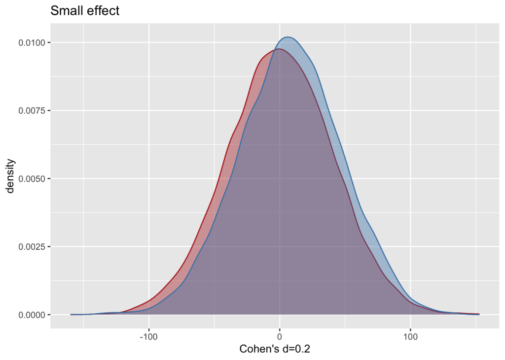
Plot the three typical effect sizes
es.labs <- c("Small", "Medium", "Large")
es.d <- c(0.2, 0.5, 0.8)
es.ss <- c(400, 65, 25)
plots <- vector("list", length(es.d))

for ( i in 1:3) {
  m1 <- 0; sd <- 40; #sample 1 mean and standard deviation
  d <- es.d[i]; #Cohen's d
  m2 <- m1 + d * sd; #sample 2
  n <- es.ss[i]; #sample size (i.e. the number of pairs, or the number in each group)
  df <- data.frame(pop1 = rnorm(n, m1, sd), pop2 = rnorm(n, m2, sd))
  g <- ggplot (df) +
    geom_density(aes(x=pop1), color="firebrick", fill="firebrick", alpha=0.4) +
    geom_density(aes(x=pop2), color="steelblue", fill="steelblue", alpha=0.4) +
    labs(x= paste0("Cohen's d=",d), title=paste(es.labs[i], "effect"))
  plots[[i]] <- g
}
gridplots(plots, 3)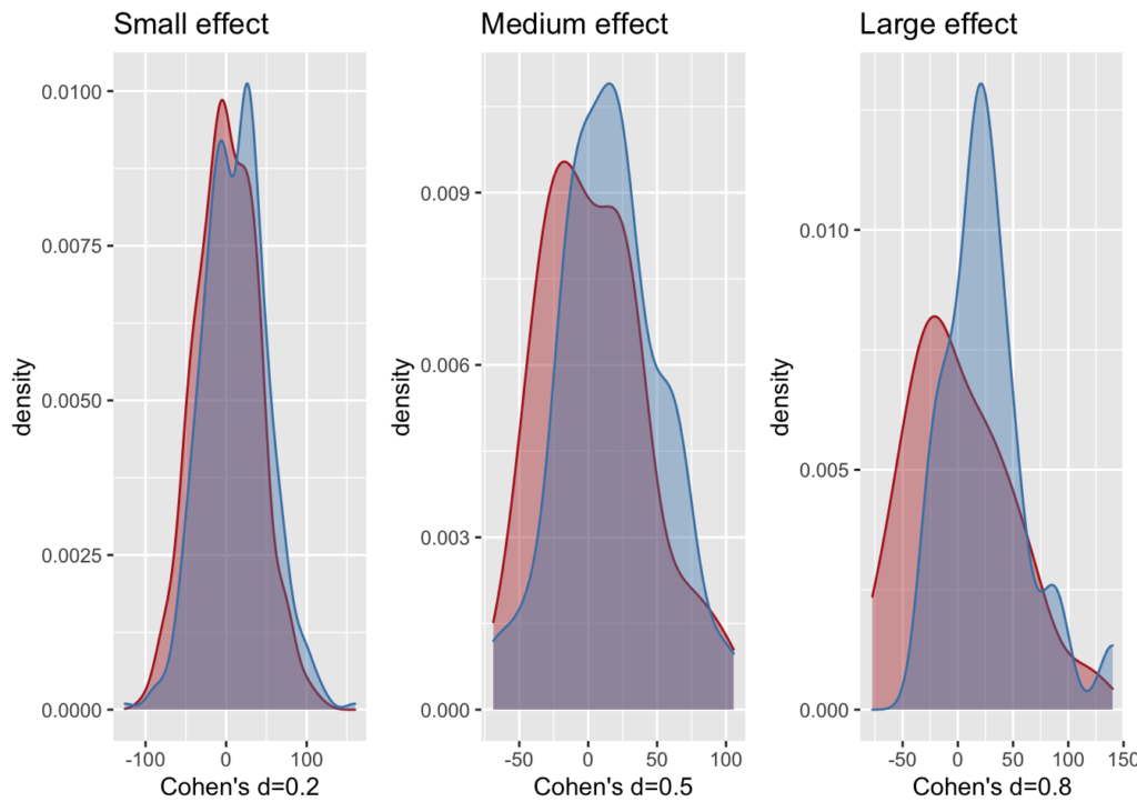
Calculate Cohen’s d for two groups with different standard deviations
From Salvatore S. Mangiafico An R Companion for the Handbook of Biological Statistics
### --------------------------------------------------------------
### Power analysis, t-test, student height, pp. 43–44
### --------------------------------------------------------------

M1  = 66.6                      # Mean for sample 1
M2  = 64.6                      # Mean for sample 2
S1  =  4.8                      # Std dev for sample 1
S2  =  3.6                      # Std dev for sample 2

Cohen.d = (M1 - M2)/sqrt(((S1^2) + (S2^2))/2)

pwr.t.test(
       n = NULL,                  # Observations in _each_ group
       d = Cohen.d,
       sig.level = 0.05,          # Type I probability
       power = 0.80,              # 1 minus Type II probability
       type = "two.sample",       # Change for one- or two-sample
       alternative = "two.sided"
       )
##
## Two-sample t test power calculation
##
## n = 71.61288
## d = 0.4714045
## sig.level = 0.05
## power = 0.8
## alternative = two.sided
##
## NOTE: n is number in *each* groupWhat fraction of studies is significant to p<0.05?
In other words, what is the power? n=number of pairs, s= num of studies/simulations; d=Cohen’s d. Let’s make a function to simplify repetitive procedures.
proportion_significant <- function (s, n, d, alpha, beta, returnVector){
    if(missing(alpha)) alpha <- 0.05
    if(missing(beta)) beta   <- 0.8
    if(missing(d)) d <- 0.2 #Small difference; 0.5=medium; 0.8=large
    if(missing(n)) {
        library(pwr)
        n <- pwr.t.test(d=d, sig.level=alpha, power=beta, type="two.sample")$n
    }
    if(missing(returnVector)){returnVector = FALSE}
    if(missing(s)) s <- 30
  p_value_vector <- c()
  for (i in 1:s) {  #s is the number of studies, e.g. 1000
    #if (i %% 100 if == 0) {cat(i)} else {cat(".")}
    df <- data.frame(a = rnorm(n, m1, sd), b = rnorm (n, m1 + d * sd, sd))
    p_value_vector <- c(p_value_vector, t.test(df$a, df$b)$p.value )
    i <- i+1
  }
  p <- data.frame(p=p_value_vector); head(p)
  p <- p[order(p$p),]
  p <- data.frame(x=1:s,p=p); p
  power_count <- length(subset(p$p, p$p < alpha));
  proportion_significant <- power_count/s ; proportion_significant
  if (returnVector == TRUE) {
    return(p[,-1])}
  else {
    return(proportion_significant)
  }
}
proportion_significant(s=30, n=360, d=0.2) # changes every time
## [1] 0.8333333Plot power
As function of n (=no of pairs) and d (=diff bet means)
n <- 400
df <-  data.frame(x=seq(5, n, 5))
df$small <- sapply(df$x, FUN=function(x){proportion_significant(k, x, 0.2, alpha,beta)})
df$medium <- sapply(df$x, FUN=function(x){proportion_significant(k, x, 0.5, alpha,beta)})
df$large <- sapply(df$x, FUN=function(x){proportion_significant(k, x, 0.8, alpha,beta)})
ggplot(df)  +
    geom_smooth(aes(x=x, y=small), color = "darkgray") +
    geom_smooth(aes(x=x, y=medium), color = "steelblue") +
    geom_smooth(aes(x=x, y=large), color = "firebrick") +
    geom_hline(yintercept = beta) +
    scale_y_continuous(limits = c(0, 1.05), breaks=seq(0,1,0.1)) +
    scale_x_continuous(limits = c(0, n), breaks=seq(0, n, 25)) +
    ggtitle("Cohen's d = small (gray); medium (blue); large (red)") +
    ylab("Power") + xlab("Number of pairs")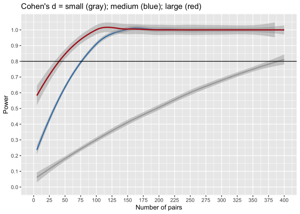
Solve the sample size
d <- 0.5; # Cohen's d
k <-100;  # no of simulations
alpha <- 0.05; beta <- 0.8; m1 <- 0; sd <- 10; #mean and standard deviation for sample_1
# power function
pf <- function(d) {
    return(pwr.t.test(d=d, sig.level=alpha, power=beta, type="two.sample")$n)
    }
pf(0.1)
## [1] 1570.733x <- seq (0.2, 0.8, 0.025) #d values
df <- data.frame(d=x,
n=sapply(x, FUN=function(x){pf(d=x)}))
ggplot(df) +
geom_smooth(aes(x=d, y=n), color="gray") +
geom_point(aes(x=d, y=n), color="firebrick4", size=4, alpha=I(2/3)) +
#geom_hline(yintercept = f(0.2)) +
#geom_hline(yintercept = f(0.5)) +
#geom_hline(yintercept = f(0.8)) +
scale_y_continuous(limits = c(0, 400), breaks=seq(0,400,20)) +
scale_x_continuous(limits = c(0.2, .8), breaks=seq(0.2, .8, 0.05)) +
ggtitle("Sample size as function of Cohen's d") +
ylab("n (# of pairs)") + xlab("Cohen's d")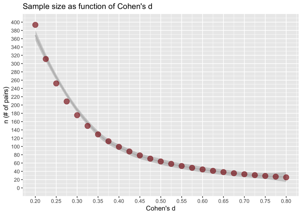
Not plotted above is pf(0.1)=1570.733, at which point you can probably prove statistical significance, but you should ask yourself if the difference is practically significant.
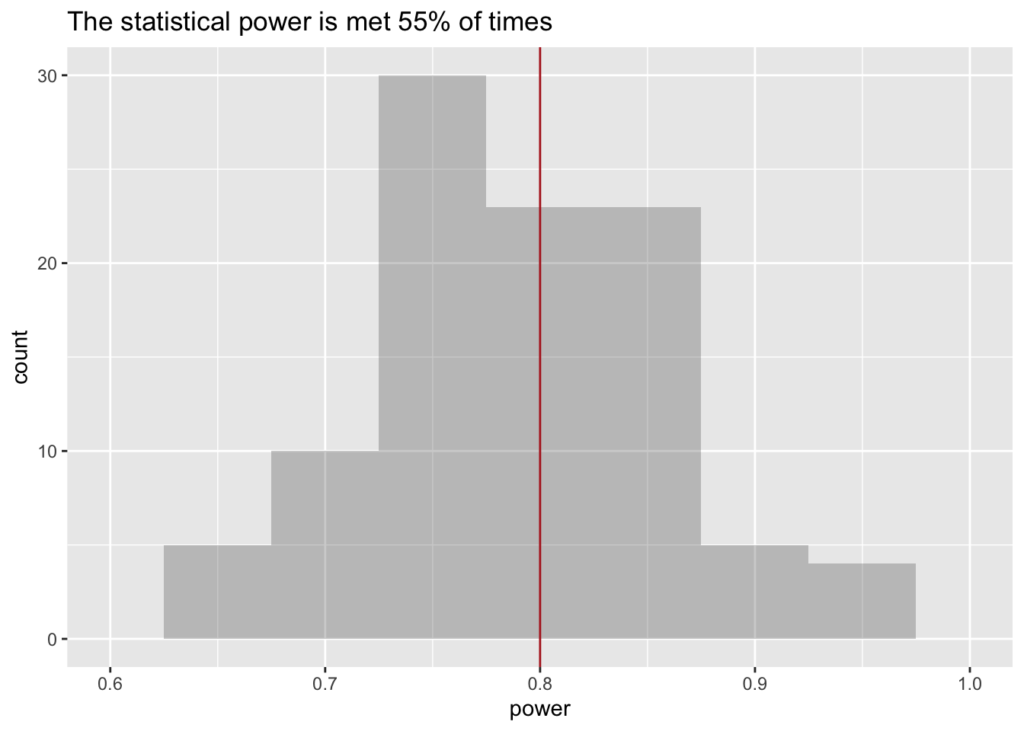
How many studies cross the 80% threshold?
Even a study sized properly (i.e. following a power calculation) will not always guarantee that it is not underpowered. That is because the power calculation only promises that you have the righ size on average. Let’s plot the histogram of power distribution.
Assuming large effect (d=0.8) and n=25 (appropriate for power=0.8)
s <- 30;  d <- 0.8; n <- 25; #alpha <- 0.05; beta = 0.8
df <- replicate (100, proportion_significant(s, n, d));
df <- data.frame(power=df[order(df)])
ldb <-length(subset(df$power, df$power>=beta))/nrow(df); #ldb #what fraction > beta
ggplot(df) +
    geom_histogram(aes(x=power), binwidth=prettyb(df$power), alpha=I(0.3)) +
    scale_x_continuous(limits = c(floor(min(df$power)*10)/10,
                                  ceiling(max(df$power)*10)/10)) +
    geom_vline(xintercept=0.8, color="firebrick") +
    labs(title = paste0 ("The statistical power is met ", round(ldb*100), "% of times"))