Bootstraping

Bootstrapping (or ‘the bootstrap’) is a statistical technique of drawing repeated samples (resampling) with replacement from an available sample; this ultimately allows one to draw inferences about a population from the available sample. The number of resamples is usually large (say, 10,000), although with a representative sample, 50 resamples will get you there.

This is an example with 30 resamples (speed up the video manually after the first sample):

And here is an example of bootstrapping a linear regression:

NOTE: would happily give credit to the author of these videos that I saved from the web a long time ago, so if you know who they are, write in a comment below!

And now let’s play in R!

suppressMessages(suppressWarnings(sapply(c("ggplot2",  "rms", "boot", "kbtools"), require, character.only = T)))
options(scipen=5, warn=0) 
n <- 100; df <- betac(c(0.8, 0.6, 0.9), n); names(df) <- "lab"; df$age = rnorm(n,50,10);
ggplot(df) + geom_histogram(aes(x=lab), fill="steelblue") + scale_x_continuous(lim=c(0.6,.9))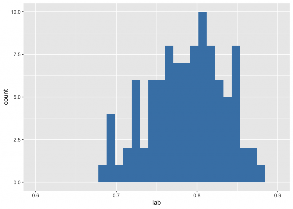

Let’s estimate the mean of age. The bootstrap function must always look like this:

ma <- function(data,i){ # must have 2 args
    data <- data[i,]    # must look like this
    mean(data$age)}     # your function
bs <- boot(df, ma, 1000); #bs; summary(bs)
ci <- boot.ci(bs, type= "bca")
paste0("mean:", format(mean(bs$t), digits=4),
       ", sd:", format(sd(bs$t), digits=4),
       " (95%CI ",format(ci$bca[4], digits=4),"-",format(ci$bca[5], digits=4),")")

## [1] "mean:50.99, sd:0.9243 (95%CI 49.12-52.69)"

Let’s estimate the median of lab

ml <- function(data,i){ #must have 2 args
    data <- data[i,] #must look like this
    median (data$lab)}
bs <- boot(df, ml, 1000); #bs; 
ci <- boot.ci(bs, type= "bca")
paste0("median:", format(mean(bs$t), digits=4),
       ", sd:", format(sd(bs$t), digits=4),
       " (95%CI ",format(ci$bca[4], digits=4),"-",format(ci$bca[5], digits=4),")")

## [1] "median:0.792, sd:0.006542 (95%CI 0.7782-0.8021)"

plot(bs)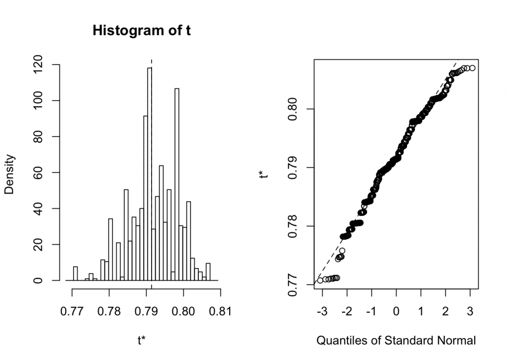

Get a small sample from a population and estimate the population mean

n <- 100000; pop <- betac(c(0.8, 0.6, 0.9), n); names(pop) <- "lab"; pop$age = rnorm(n,50,10);

##  num [1:3] 0.8 0.6 0.9

ggplot(pop) + geom_histogram(aes(x=age), fill="steelblue")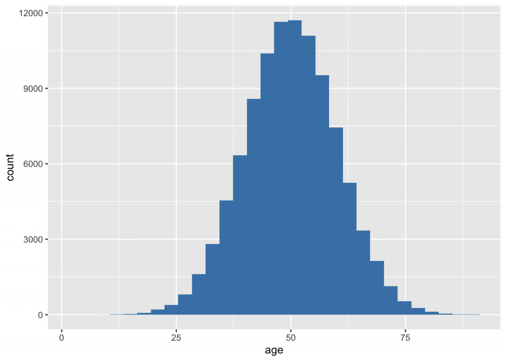

k <- 20; s <- sample(1:n, k, replace = F)  #small sample
sa <- pop[s,]; head(sa); #mean(sa$age); mean(pop$age)

##             lab      age
## 38751 0.6647264 63.70903
## 59115 0.7926795 69.24643
## 50179 0.7825356 66.93178
## 99763 0.7748456 67.58385
## 87572 0.8217341 46.74479

#bootstrap age
bs <- boot(sa, ma, n); head(bs$t)

##          [,1]
## [1,] 53.49271
## [2,] 47.60810
## [3,] 51.78993
## [4,] 55.26985
## [5,] 51.02422
## [6,] 53.65478

pop$age.bs <- bs$t

cia <- boot.ci(bs, type= "bca")
r <- sort(bs$t); iqr <- c(r[round(n*.25)], r[round(n*.75)]); iqr #brute force  IQR

## [1] 50.99627 54.28866

paste0("Age  mean (95%CI): ", format(mean(bs$t), digits=5), # "; sd:", format(sd(bs$t), digits=4),
       " (", format(cia$bca[4], digits=5),"-",format(cia$bca[5], digits=5),")",
       ";  median (IQR): ", format(median(bs$t), digits=5), " (", format(iqr[1], digits=5), "-", format(iqr[2], digits=5), ")")

## [1] "Age  mean (95%CI): 52.657 (48.119-57.616);  median (IQR): 52.628 (50.996-54.289)"

##lab
bs <- boot(sa, ml, n);
pop$lab.bs <- bs$t
#display info
cil <- boot.ci(bs, type= "bca")
r <- sort(bs$t); iqr <- c(r[round(n*.25)], r[round(n*.75)]); iqr #brute force  IQR

## [1] 0.7926795 0.8066732

paste0("mean (95%CI): ", format(mean(bs$t), digits=5), # "; sd:", format(sd(bs$t), digits=4),
       " (", format(cil$bca[4], digits=5),"-",format(cil$bca[5], digits=5),")",
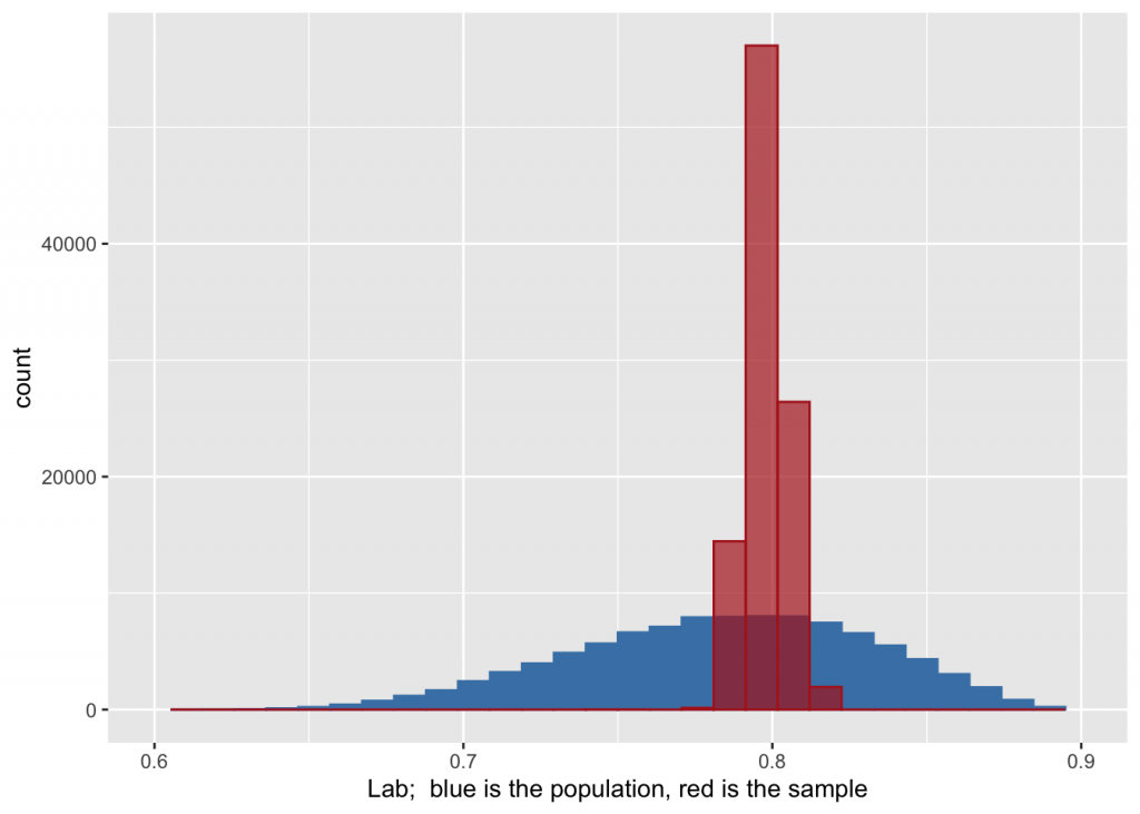
       ";  median (IQR): ", format(median(bs$t), digits=5), " (", format(iqr[1], digits=5), "-", format(iqr[2], digits=5), ")")

## [1] "mean (95%CI): 0.79841 (0.78761-0.81062);  median (IQR): 0.79651 (0.79268-0.80667)"

pop$lab.bs <- bs$t

g <- ggplot(pop) 
g + geom_density(aes(x=age), color="steelblue", fill="steelblue") +  geom_density(aes(x=age.bs), alpha=I(0.7), color="firebrick", fill="firebrick") + labs(x=paste("Age; ", "blue is the population, red is the sample"))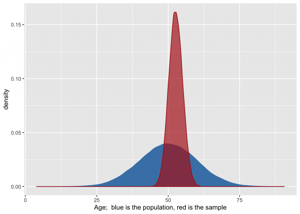

g + geom_histogram(aes(x=lab), color="steelblue", fill="steelblue") + geom_histogram(aes(x=lab.bs), alpha=I(0.7), color="firebrick", fill="firebrick") + labs(x=paste("Lab; ", "blue is the population, red is the sample")) + scale_x_continuous(lim=c(0.6,0.9))

Leave a Reply Cancel reply