- Definition
- Informative vs. uninformative priors
- Mean, median, variance
- Highest Density Interval
- References
- Addenda
Definition
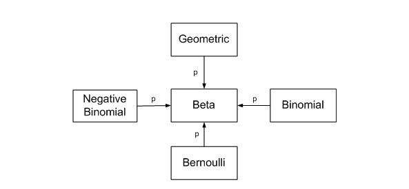
The Beta distribution represents a probability distribution of probabilities. It is the conjugate prior of the binomial distribution (if the prior and the posterior distribution are in the same family, the prior and posterior are called conjugate distributions) (Figure from John Cook’s blog).
Using the mean
As an example, the MLB’s all-time league batting average (number of “hits” divided by “at bats”) is between .260 and .275. For this discussion we will start with an average of 0.27. THe beta distribuition’s moments alpha and beta are the probabilities of success and failure. The probability of success in 300 trials is represented graphicaly by a beta distribution with alpha = 300*0.27 and beta = 300*(1-0.27):
n <- 300   # no of Bernoulli trials
ba <- 0.27 # batting avg
g <- ggplot(data.frame(z=c(0,1)), aes(x=z))
g + stat_function(fun = dbeta, args= list(shape1=n*ba, shape2=n*(1-ba)), color="steelblue")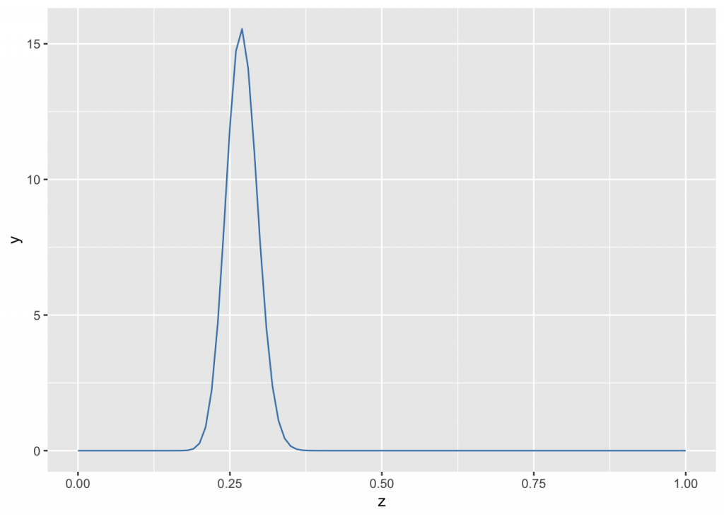
The \(y\) axis shows the probability per unit of x, so it is a probability density. In Bayesian analysis, the prior need not be beta-distributed only the likelihood must be beta distributed. If beta-distributed, individual points on the \(y\) axis can be any positive value as long as the area under the curve integrates to 1.
Back to baseball. At the beginning of the season, after five pitches with four hits, one might naïvely say the player’s success rate is 80%. When factored against the prior, however, the probability changes only slightly.
g +
    stat_function(fun = dbeta, args=list(81, 219), color="steelblue", size=1) +
    stat_function(fun = dbeta, args=list(85, 220), color="firebrick", size=1) +
    annotate("text", x=0.175, y=14.7, label="before", color="steelblue") +
    annotate("text", x=0.37,  y=14.7, label="after",  color="firebrick")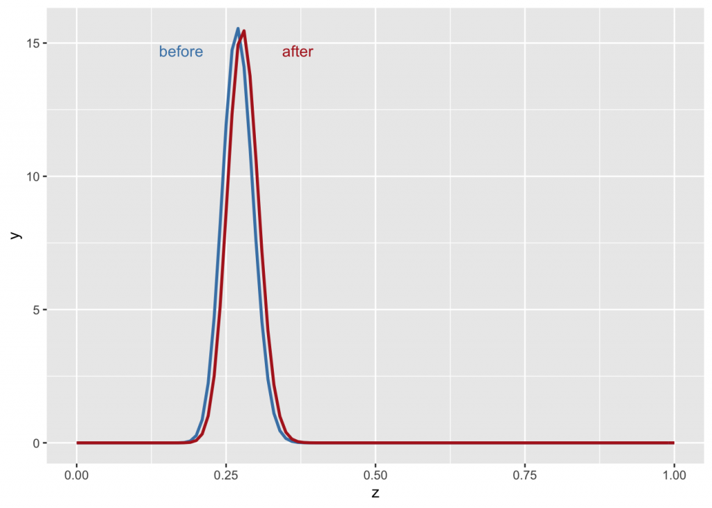
So far, then, we have:
- defined the prior distribution that incorporates our subjective beliefs about a parameter (historical batting averages).
- gathered data.
- updated the prior distribution with the data using Bayes’ theorem to obtain a posterior distribution (for the posterior, you basically just add up the hits and misses).
The posterior distribution is a probability distribution that represents the updated beliefs about the parameter after having seen the data. This is the essence of bayesian statistics, based on Bayes’ theorem \[posterior\hspace{4pt}\alpha \hspace{4pt}prior*likelihood\]
Using ranges for the prior
Another way to use the knowledge that MLB’s all-time league batting average (number of “hits” divided by “at bats”) is between .260 and .275 is to say we are 95% sure the averages will fall between these two numbers. We will use the library LearnBayes for this exercise:
quantile1=list(p=.025,x=0.24) ##there was some error if 0.26
quantile2=list(p=.975,x=0.280) #can be other beliefs, like median, 90th perc etc
beta.select(quantile1,quantile2)
## [1] 481.14 1371.51alpha <- beta.select(quantile1,quantile2)[[1]]
beta <- beta.select(quantile1,quantile2)[[2]]If you are less sure of your prior, reduce your parameters proportionally:
g +
    stat_function(fun = dbeta, args=list(alpha, beta), color="steelblue", size=1) +
    stat_function(fun = dbeta, args=list(alpha/10, beta/10), color="orange", size=1) +
    annotate("text", x=0.4,  y=1, label="smaller sample",  color="orange")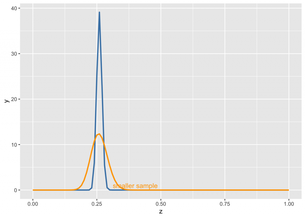
Informative vs. uninformative priors
An uninformative uniform prior is when there is no knowledge, so any probability is equally likely (the prior is flat). Priors are rarely completely uninformative, hence the concept of weakly informative priors (Lambert p 255). Nevertheless, let’s say the player had 4 hits out of of 20 tries.
g +
    stat_function(fun = dbeta, args=list(1, 1), color="steelblue", size=1) +
    stat_function(fun = dbeta, args=list(4, 16), color="green", size=1) +
    stat_function(fun = dbeta, args=list(5, 17), color="firebrick", size=1) +
    labs(title="Uninformative prior") +
    annotate("text", x=0.5,  y=1.1, label="prior",  color="steelblue") +
    annotate("text", x=0.09,  y=3.9, label="data",  color="green") +
    annotate("text", x=0.31,  y=3.6, label="posterior",  color="firebrick")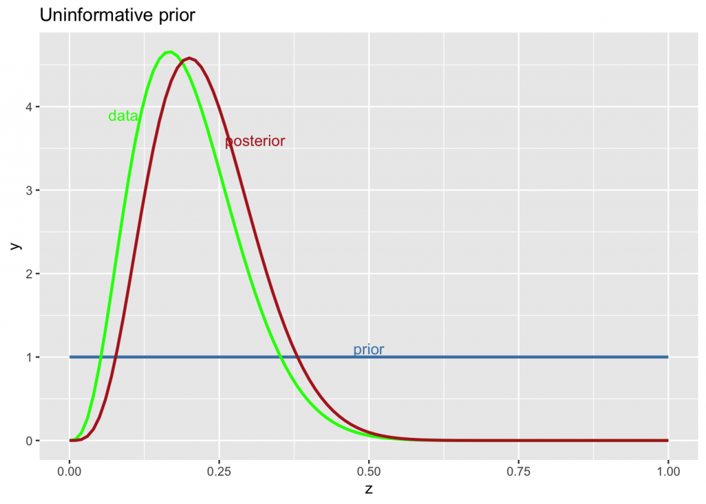
The posterior is completely determined by the likelihood.
Jeffrey’s priors can be used in such a situation. Although a mathematical form is available, a beta (.5, .5) is a convenient form, that is strictly accurate in the case of a Bernoulli distribution (a special case of the binomial distribution)
curve(dbeta(x, .5, .5), from=0, to=1)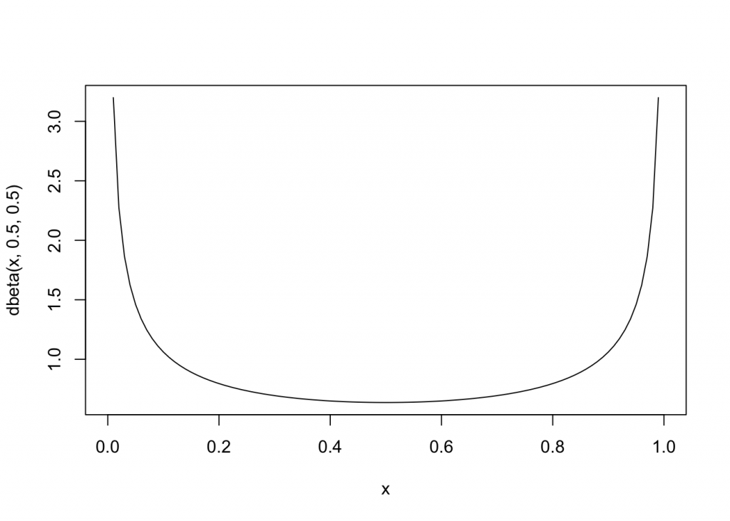
On the other hand, if the knowledge is drawn from a large sample size, the prior is highly informative
n <- 300
g +
    stat_function(fun = dbeta, args=list(n*0.27, n*(1-0.27)), color="steelblue", size=1)  +
    stat_function(fun = dbeta, args=list(4, 16), color="green", size=1) +
    stat_function(fun = dbeta, args=list(n*0.27+4, n*(1-0.27)+16), color="firebrick", size=1) +
    labs(title="Highly informative prior")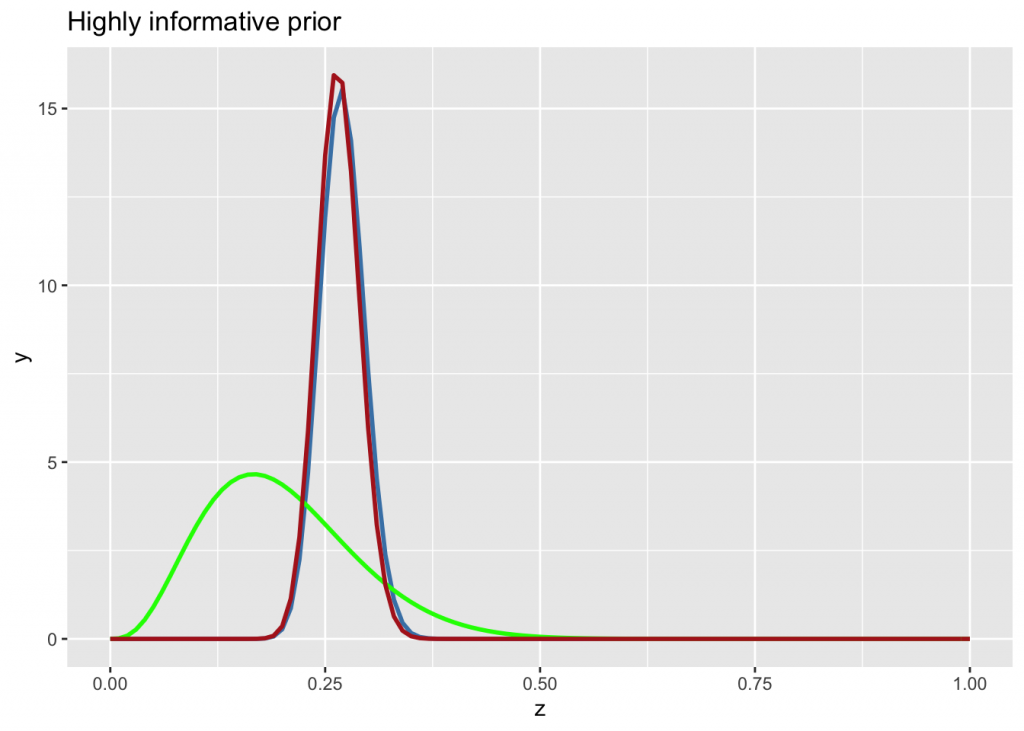
The posterior is completely determined by the prior.
If the prior is derived from a small sample (e.g. n=10), the data will overwhelm it if the observation sample is big (say 100 trials). The posterior will be a beta distribution with \(\alpha =\) 2.7 + 18 and \(\beta =\) 7.3 + 82.
n <- 10
g +
    stat_function(fun = dbeta, args=list(n*0.27, n*(1-0.27)), color="steelblue", size=1) +
    stat_function(fun = dbeta, args=list(18, 82), color="green", size=1) +
stat_function(fun = dbeta, args=list(n*0.27 + 18, n*(1-0.27) + 82), color="firebrick", size=1) 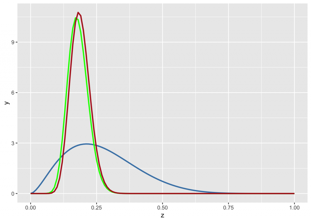
Mean, median, variance
The expected value (mean) of the beta distribution is \[ \frac{\alpha }{\alpha + \beta}\] or in the case of \(\alpha\)=81 and \(\beta\)=219, the batting average. The mode is \[\frac {\alpha-1}{\alpha + \beta -2}\] which, in this case is 81.5402685. The median does not have a closed form, but can be approximated as \[median \approx \frac{\alpha – \frac{1}{3}}{\alpha + \beta – \frac{2}{3}} \hspace{4pt} for \hspace{4pt}\alpha , \beta \geq 1\] The variance is \[ var(X) = \frac{\alpha \beta}{(\alpha + \beta)^2(\alpha + \beta + 1)}\]
Highest Density Interval
In asymmetric sitributions, the 95% highest density interval (HDI) of the posterior is different than the 2.5- and 97.5 percentiles, and can be calculated with the HDInterval library. For a 95% HDI, 10,000 independent draws are recommended; a smaller number will be adequate for a 80% HDI, many more for a 99% HDI. The library HDInterval is needed here.
alpha <- 27; #n*0.27 + 18; alpha
beta <- 83; #*(1-0.27) + 82; beta
s<-seq(0, 1, length=10001); #s
db<- dbeta(s, alpha, beta);  #plot(db) ; #db;
low <- qbeta(0.025, alpha, beta); ##dbeta(low, alpha, beta)
hi  <- qbeta(0.975, alpha, beta); ##dbeta(hi, alpha, beta)
qbeta(c(0.025,0.975), alpha, beta)
## [1] 0.1700199 0.3296520my.hdi <- hdi(qbeta(s, alpha, beta), 0.95); my.hdi #HDI uses qbeta## lower upper
## 0.1671799 0.3263479
## attr(,"credMass")
## [1] 0.95hdi.low <- my.hdi[[1]]; #hdi.low
hdi.hi <- my.hdi[[2]]; #hdi.hi
y.hdi.low <- dbeta(hdi.low, alpha, beta); #y.hdi.low
y.hdi.hi <- dbeta(hdi.hi, alpha, beta); #y.hdi.hi
g +
stat_function(fun = dbeta, args=list(alpha, beta), color="steelblue") +
geom_segment(x=low, xend=hi, y=1.10, yend=1.10, color="black") +
geom_segment(x=hdi.low, xend=hdi.hi, y=y.hdi.low, yend=y.hdi.hi, color="firebrick", size=1) +
annotate("text", x=0.4, y=1.46, label="95% HDI", color="firebrick")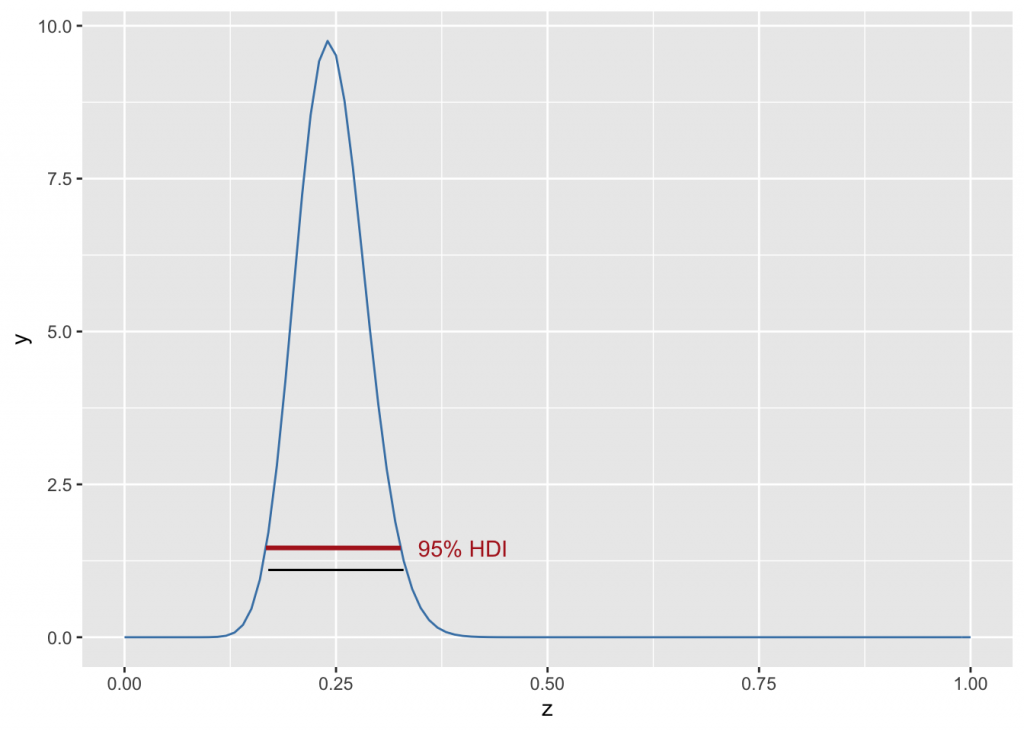
References
- DataSciFact
- John Cook’s blog
- B Lambert: A Student’s Guide to Bayesian Statistics
- CrossValidated: What is the intuition behind beta distribution?
- CrossValidated: Help me understand Bayesian prior and posterior distributions
Addenda
- The Bayes’s equation above shows that one adds blank spaces in \(\LaTeX\) by using
\hspace{4pt}#RMarkdown #Latex
- To add inline R code that is evaluated use “‘r code’” (\(\sqrt 2\)=1.4142136), otherwise, for highlighting just use the left ’
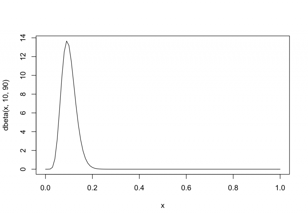
code - The function
curveis an easy way to plot a function passing a parameterx
curve(dbeta(x, 10, 90), from=0, to=1)