MLE – The Maximum Likelihood Estimate

The maximum likelihood estimation (MLE) is a general method to find the function that most likely fits the available data; it therefore addresses a central problem in data sciences.

Depending on the model, the math behind MLE can be very complicated, but an intuitive way to think about it is through the following thought experiment. You are given two urns, the first with 9 red balls and one white ball, and the second, containing the reverse(9 white balls and one red). The urns are behind a curtain and you cannot see them, but can reach both of them equally well. Their location (order) is then shuffled and the balls in each urn are also shuffled. Thus blinded, you reach into one of the urns and draw one ball. If the ball is white, you will probably conclude that you drew from the second urn, because that reasoning maximizes the likelihood, given the experimental data.

Another way to think about MLE (and frequentist NHST) is illustrated in this cartoon:

Maximum likelihood is a very general approach that can be used to fit many models. For example, in logistic regression, non-linear least squares could be used to fit the model, but it is vastly more common to use MLE to find the parameters. In fact, the least squares approach is a special case of MLE (James, p133).

The generic mathematical way to express the likelihood function is \[L(\mu|X) =\prod_{i=1}^{N}f(x_i,\mu)\] which is transformed as log-likelihood, because of the latter’s more desirable properties \[\ln L(\mu|X)=\sum_{i=1}^{N}\ln f(x_i,\mu)\]

Optimizers (such as the nlm function from the stats package) typically minimize a function, so we use the negative log-likelihood for minimizing, and that is equivalent to maximizing the log-likelihood or the likelihood itself. The deviance of a logistic regression model is a measure of goodness-of-fit and is equivalent to the sums of squares in OLS, although it is calculated differently (Cohen, p 499). The statistical tests built on deviance are collectively referred to as likelihood ratio tests, and a common notation for deviance is \(-2LL\) or -2 log likelihood \[Deviance = -2\hspace{4pt}ln(likelihood \hspace{4pt}ratio) = -2\hspace{4pt}ln\frac{ML_{under \hspace{4pt}one \hspace{4pt}model}}{ML_{under \hspace{4pt}more \hspace{4pt}complete \hspace{4pt}model}} \]

Let’s use the function optimize from the package stat first

set.seed(123)
x <- rnorm(100, 2.71) # a normal distribution with mu=2.71 

The likelihood function is the product of all \(f(x_i, \mu)\), or the sum of all \(ln(f(x_i, \mu))\), where the function is dnorm(x, mu)

loglik <- function(mu) sum(log(dnorm(x, mu)))

Will apply that over an arbitrary range

data.ll <- vapply(seq(-6, 6, by=0.001), loglik, numeric(1))
plot(seq(-6, 6, by=0.001), data.ll, type="l", ylab="Log-Likelihood", xlab=expression(mu))
abline(v=mean(x), col="red")

Next we optimize the function to find its maximum

optimize(loglik, interval=c(-6, 6), maximum=TRUE)$maximum

## [1] 2.800406

Exercise 2

Given n numbers assumed to come from a normally distributed population we will estimate the parameters of the original distribution.

set.seed(53)
n <- 10
sample <- rnorm (n, 32, 12);  

We will guess (err, use domain expertise) that the mean mu will be somewhere between 20 and 60 and sd will be between 9 and 16.

tol <-.05 #arbitrary level of tolerance
mu <- seq (20, 60, by=tol);  #length(mu); #mu;
sd <- seq (9, 16, by=tol);  #length(sd); #sd;

And calculate the log-likelihood for each pair (mu, sd):

loglik <- function(mu, sd) (sum(log(dnorm(sample, mu, sd)))) 
m <-  sapply(mu,  function(x) sapply(sd, function(y) loglik(x,y)))
dimnames(m) <- list(sd, mu) #str(m)

The apply function make this calculation MUCH faster than if using loops, and the above is a beautiful example of a nested, multidimensional apply. Next we will find the maximum log likelihood (ie. optimize the function).

mx <- which (m == max(m), arr.ind = T); max(m); mx

## [1] -39.22094

##      row col
## 12.2  65 240

mu[mx[2]] #mle for mu

## [1] 31.95

sd[mx[1]] #mle for sd

## [1] 12.2

image.plot(matrix((data=m), ncol=length(mu), nrow=length(sd)), nlevel=64)
abline (h=(mu[mx[2]]-range(mu[1]))/(range(mu)[2]-range(mu)[1]))
abline(v=(sd[mx[1]]-range(sd[1]))/(range(sd)[2]-range(sd)[1]))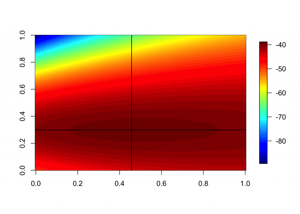

Using the function nlm

Another way to do MLE in R is with the function nlm that minimizes arbitrary functions written in R.

X <- c(rep(0,14), rep(1,30), rep(2,36), rep(3,68), rep(4, 43), rep(5,43), rep(6, 30), rep(7,14),
rep(8,10), rep(9, 6), rep(10,4), rep(11,1), rep(12,1))
#hist(X, main="histogram of number of right turns", right=FALSE, prob=TRUE)
n <- length(X); n

## [1] 300

negloglike <- function(lam) { n* lam -sum(X) *log(lam) + sum(log(factorial(X))) }
negloglike(0.3)

## [1] 2583.046

out<-nlm(negloglike, p=c(0.5), hessian = TRUE); out

## $minimum
## [1] 667.183
## 
## $estimate
## [1] 3.893331
## 
## $gradient
## [1] -2.569636e-05
## 
## $hessian
##          [,1]
## [1,] 77.03948
## 
## $code
## [1] 1
## 
## $iterations
## [1] 10

f <- function(x) sum((x-1:length(x))^2)
nlm(f, c(10,10))

## $minimum
## [1] 4.303458e-26
## 
## $estimate
## [1] 1 2
## 
## $gradient
## [1]  2.757794e-13 -3.099743e-13
## 
## $code
## [1] 1
## 
## $iterations
## [1] 2

#nlm(f, c(10,10), print.level = 2)
utils::str(nlm(f, c(5), hessian = TRUE))

## List of 6
##  $ minimum   : num 2.44e-24
##  $ estimate  : num 1
##  $ gradient  : num 1e-06
##  $ hessian   : num [1, 1] 2
##  $ code      : int 1
##  $ iterations: int 1

f <- function(x, a) sum((x-a)^2)
nlm(f, c(10,10), a = c(3,5))

## $minimum
## [1] 3.371781e-25
## 
## $estimate
## [1] 3 5
## 
## $gradient
## [1]  6.750156e-13 -9.450218e-13
## 
## $code
## [1] 1
## 
## $iterations
## [1] 2

f <- function(x, a) {
    res <- sum((x-a)^2)
    attr(res, "gradient") <- 2*(x-a)
    res
}
nlm(f, c(10,10), a = c(3,5))

## $minimum
## [1] 0
## 
## $estimate
## [1] 3 5
## 
## $gradient
## [1] 0 0
## 
## $code
## [1] 1
## 
## $iterations
## [1] 1

f <- function (x) (-x^2 +5)
nlm (f, p=c(0), hessian = T)

## $minimum
## [1] 5
## 
## $estimate
## [1] 0
## 
## $gradient
## [1] -1.000089e-06
## 
## $hessian
##      [,1]
## [1,]   -2
## 
## $code
## [1] 1
## 
## $iterations
## [1] 0

demo(nlm)

## 
## 
##  demo(nlm)
##  ---- ~~~
## 
## > #  Copyright (C) 1997-2009, 2017 The R Core Team
## > 
## > ### Helical Valley Function
## > ### Page 362 Dennis + Schnabel
## > 
## > require(stats); require(graphics); require(utils)
## 
## > theta <- function(x1,x2) (atan(x2/x1) + (if(x1 <= 0) pi else 0))/ (2*pi)
## 
## > ## but this is easier :
## > theta <- function(x1,x2) atan2(x2, x1)/(2*pi)
## 
## > f <- function(x) {
## +     f1 <- 10*(x[3] - 10*theta(x[1],x[2]))
## +     f2 <- 10*(sqrt(x[1]^2+x[2]^2)-1)
## +     f3 <- x[3]
## +     return(f1^2 + f2^2 + f3^2)
## + }
## 
## > ## explore surface {at x3 = 0}
## > x <- seq(-1, 2, length.out=50)
## 
## > y <- seq(-1, 1, length.out=50)
## 
## > z <- apply(as.matrix(expand.grid(x, y)), 1, function(x) f(c(x, 0)))
## 
## > contour(x, y, matrix(log10(z), 50, 50))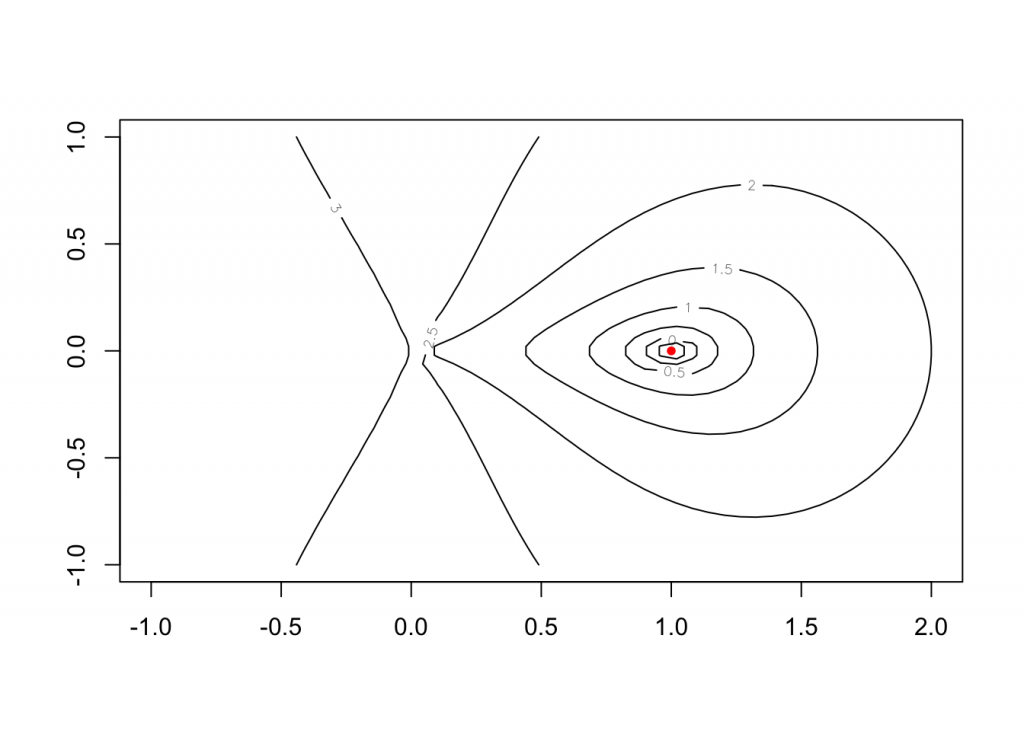

## 
## > str(nlm.f <- nlm(f, c(-1,0,0), hessian = TRUE))
## List of 6
##  $ minimum   : num 1.24e-14
##  $ estimate  : num [1:3] 1.00 3.07e-09 -6.06e-09
##  $ gradient  : num [1:3] -3.76e-07 3.49e-06 -2.20e-06
##  $ hessian   : num [1:3, 1:3] 2.00e+02 -4.07e-02 9.77e-07 -4.07e-02 5.07e+02 ...
##  $ code      : int 2
##  $ iterations: int 27
## 
## > points(rbind(nlm.f$estim[1:2]), col = "red", pch = 20)
## 
## > stopifnot(all.equal(nlm.f$estimate, c(1, 0, 0)))
## 
## > ### the Rosenbrock banana valley function
## > 
## > fR <- function(x)
## + {
## +     x1 <- x[1]; x2 <- x[2]
## +     100*(x2 - x1*x1)^2 + (1-x1)^2
## + }
## 
## > ## explore surface
## > fx <- function(x)
## + {   ## `vectorized' version of fR()
## +     x1 <- x[,1]; x2 <- x[,2]
## +     100*(x2 - x1*x1)^2 + (1-x1)^2
## + }
## 
## > x <- seq(-2, 2, length.out=100)
## 
## > y <- seq(-0.5, 1.5, length.out=100)
## 
## > z <- fx(expand.grid(x, y))
## 
## > op <- par(mfrow = c(2,1), mar = 0.1 + c(3,3,0,0))
## 
## > contour(x, y, matrix(log10(z), length(x)))

## 
## > str(nlm.f2 <- nlm(fR, c(-1.2, 1), hessian = TRUE))
## List of 6
##  $ minimum   : num 3.97e-12
##  $ estimate  : num [1:2] 1 1
##  $ gradient  : num [1:2] -6.54e-07 3.34e-07
##  $ hessian   : num [1:2, 1:2] 802 -400 -400 200
##  $ code      : int 1
##  $ iterations: int 23
## 
## > points(rbind(nlm.f2$estim[1:2]), col = "red", pch = 20)
## 
## > ## Zoom in :
## > rect(0.9, 0.9, 1.1, 1.1, border = "orange", lwd = 2)
## 
## > x <- y <- seq(0.9, 1.1, length.out=100)
## 
## > z <- fx(expand.grid(x, y))
## 
## > contour(x, y, matrix(log10(z), length(x)))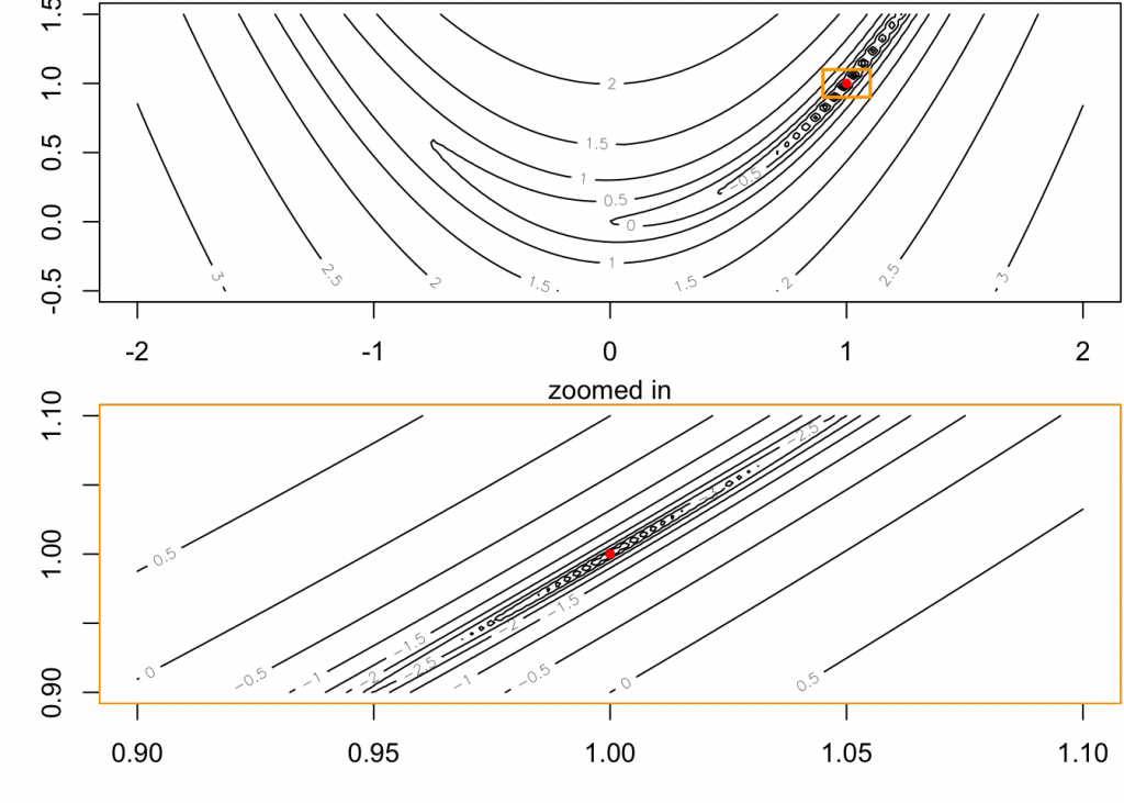

## 
## > mtext("zoomed in");box(col = "orange")
## 
## > points(rbind(nlm.f2$estim[1:2]), col = "red", pch = 20)
## 
## > par(op)
## 
## > with(nlm.f2,
## +      stopifnot(all.equal(estimate, c(1,1), tol = 1e-5),
## +                minimum < 1e-11, abs(gradient) < 1e-6, code %in% 1:2))
## 
## > fg <- function(x)
## + {
## +     gr <- function(x1, x2)
## +         c(-400*x1*(x2 - x1*x1)-2*(1-x1), 200*(x2 - x1*x1))
## +     x1 <- x[1]; x2 <- x[2]
## +     structure(100*(x2 - x1*x1)^2 + (1-x1)^2,
## +               gradient = gr(x1, x2))
## + }
## 
## > nfg <- nlm(fg, c(-1.2, 1), hessian = TRUE)
## 
## > str(nfg)
## List of 6
##  $ minimum   : num 1.18e-20
##  $ estimate  : num [1:2] 1 1
##  $ gradient  : num [1:2] 2.58e-09 -1.20e-09
##  $ hessian   : num [1:2, 1:2] 802 -400 -400 200
##  $ code      : int 1
##  $ iterations: int 24
## 
## > with(nfg,
## +      stopifnot(minimum < 1e-17, all.equal(estimate, c(1,1)),
## +                abs(gradient) < 1e-7, code %in% 1:2))
## 
## > ## or use deriv to find the derivatives
## > 
## > fd <- deriv(~ 100*(x2 - x1*x1)^2 + (1-x1)^2, c("x1", "x2"))
## 
## > fdd <- function(x1, x2) {}
## 
## > body(fdd) <- fd
## 
## > nlfd <- nlm(function(x) fdd(x[1], x[2]), c(-1.2,1), hessian = TRUE)
## 
## > str(nlfd)
## List of 6
##  $ minimum   : num 1.18e-20
##  $ estimate  : num [1:2] 1 1
##  $ gradient  : num [1:2] 2.58e-09 -1.20e-09
##  $ hessian   : num [1:2, 1:2] 802 -400 -400 200
##  $ code      : int 1
##  $ iterations: int 24
## 
## > with(nlfd,
## +      stopifnot(minimum < 1e-17, all.equal(estimate, c(1,1)),
## +                abs(gradient) < 1e-7, code %in% 1:2))
## 
## > fgh <- function(x)
## + {
## +     gr <- function(x1, x2)
## +         c(-400*x1*(x2 - x1*x1) - 2*(1-x1), 200*(x2 - x1*x1))
## +     h <- function(x1, x2) {
## +         a11 <- 2 - 400*x2 + 1200*x1*x1
## +         a21 <- -400*x1
## +         matrix(c(a11, a21, a21, 200), 2, 2)
## +     }
## +     x1 <- x[1]; x2 <- x[2]
## +     structure(100*(x2 - x1*x1)^2 + (1-x1)^2,
## +               gradient = gr(x1, x2),
## +               hessian  =  h(x1, x2))
## + }
## 
## > nlfgh <- nlm(fgh, c(-1.2,1), hessian = TRUE)
## 
## > str(nlfgh)
## List of 6
##  $ minimum   : num 1.13e-17
##  $ estimate  : num [1:2] 1 1
##  $ gradient  : num [1:2] 1.30e-07 -6.56e-08
##  $ hessian   : num [1:2, 1:2] 802 -400 -400 200
##  $ code      : int 1
##  $ iterations: int 24
## 
## > ## NB: This did _NOT_ converge for R version <= 3.4.0
## > with(nlfgh,
## +      stopifnot(minimum < 1e-15, # see 1.13e-17 .. slightly worse than above
## +           all.equal(estimate, c(1,1), tol=9e-9), # see 1.236e-9
## +           abs(gradient) < 7e-7, code %in% 1:2)) # g[1] = 1.3e-7

References:

• James et al. Intro Statistical Learning
  
• Cohen Applied Multiple Regression/Correlation Analysis for the Behavioral Sciences
  
• Examples from CrossValidated
  
• I am wondering why we use negative (log) likelihood sometimes?